Tutorial

yaf2q is a Python library for performing fermion-to-qubit mapping used in quantum chemistry calculations. It offers two main functionalities:

Performing Fermion-to-Qubit Mappings:

It supports well-known conventional methods like the Jordan-Wigner, Parity, and Bravyi-Kitaev transformations. Additionally, it supports a more generalized approach using a Ternary Tree for describing fermion-to-qubit mappings.

Optimizing Fermion-to-Qubit Mappings:

It is possible to search for a ternary tree structure that minimizes a chosen index, such as the Pauli weight in the mapped Hamiltonian, or the depth of the quantum circuit required to execute a quantum algorithm like Quantum Phase Estimation (QPE), when converting a fermionic operator to a qubit operator.

Below is a step-by-step explanation of how to use these two functionalities.

Performing Fermion-to-Qubit Mappings

Conventional Mapping Methods: Jordan-Wigner, Parity, Bravyi-Kitaev transformation

First, import the F2QMapper class, which manages the fermion-to-qubit mapping:

from yaf2q.f2q_mapper import F2QMapper

You can create an instance of F2QMapper for the conventional mappings as follows. The constructor takes the transformation method as a string and the number of qubits:

f2q_mapper = F2QMapper(kind = "jordan-wigner", num_qubits = 4)
f2q_mapper = F2QMapper(kind = "parity", num_qubits = 4)
f2q_mapper = F2QMapper(kind = "bravyi-kitaev", num_qubits = 4)

Printing the f2q_mapper (when bravyi-kitaev is specified) will show:

print(f2q_mapper)

Output:

named mapper - bravyi-kitaev (num_qubits:4)

The fermion-to-qubit mapping matrix is stored in the encoding_matrix property:

print(f2q_mapper.encoding_matrix)

Output:

[[1 0 0 0]
 [1 1 0 0]
 [0 0 1 0]
 [1 1 1 1]]

This matrix converts Fock states to qubit states. For example, the Fock state |1100) is represented as [1,1,0,0]. Applying this matrix yields [1,0,0,0], corresponding to the qubit state |1000>. While you can obtain the qubit state by matrix-multiplying the Fock state list, using the fock_to_qubit_state() method is simpler:

fock_state = [1, 1, 0, 0]
qubit_state = f2q_mapper.fock_to_qubit_state(fock_state)
print(qubit_state)

Output:

[1, 0, 0, 0]

There is also an inverse transformation method:

qubit_state = [1, 0, 0, 0]
fock_state = f2q_mapper.qubit_to_fock_state(qubit_state)
print(fock_state)

Output:

[1, 1, 0, 0]

To convert a fermion operator to a qubit operator, you first create the fermion operator using a library like OpenFermion. For instance, the fermion Hamiltonian for the H2 molecule can be created as follows:

from openfermion import MolecularData
from openfermionpyscf import run_pyscf

molecule = MolecularData(
    geometry = [('H', (0, 0, 0)), ('H', (0, 0, 0.65))],
    basis = "sto-3g",
    multiplicity = 1,
    charge = 0,
)
molecule = run_pyscf(molecule, run_scf=1, run_fci=1)
fermion_hamiltonian = molecule.get_molecular_hamiltonian()

You can then obtain the qubit operator by passing this fermion_hamiltonian to the fermion_to_qubit_operator() method:

qubit_hamiltonian = f2q_mapper.fermion_to_qubit_operator(fermion_hamiltonian)

The qubit_hamiltonian is an instance of yaf2q’s QubitOperatorSet class, which stores OpenFermion QubitOperator , qiskit SparsePauliOp or pytket QubitPauliOperator objects. These can be accessed via the openfermion_form, qiskit_form and pytket_form properties, respectively:

print(qubit_hamiltonian.openfermion_form)

Output:

03775110394645509 [] +
04407961290255181 [X0 Z1 X2] +
04407961290255181 [X0 Z1 X2 Z3] +
04407961290255181 [Y0 Z1 Y2] +
04407961290255181 [Y0 Z1 Y2 Z3] +
18601648886230604 [Z0] +
18601648886230604 [Z0 Z1] +
1699209784826151 [Z0 Z1 Z2] +
1699209784826151 [Z0 Z1 Z2 Z3] +
12584136558006329 [Z0 Z2] +
12584136558006329 [Z0 Z2 Z3] +
17297610130745106 [Z1] +
-0.26941693141631995 [Z1 Z2 Z3] +
17866777775953394 [Z1 Z3] +
-0.26941693141631995 [Z2]

print(qubit_hamiltonian.qiskit_form)

Output:

SparsePauliOp(['IIII', 'IIIZ', 'IIZI', 'IIZZ', 'IXZX', 'IYZY', 'IZII', 'IZIZ', 'IZZZ', 'ZIZI', 'ZXZX', 'ZYZY', 'ZZIZ', 'ZZZI', 'ZZZZ'],
    coeffs=[ 0.0377511 +0.j,  0.18601649+0.j,  0.1729761 +0.j,  0.18601649+0.j, 0.04407961+0.j,  0.04407961+0.j, -0.26941693+0.j,  0.12584137+0.j, 0.16992098+0.j,  0.17866778+0.j,  0.04407961+0.j,  0.04407961+0.j, 0.12584137+0.j, -0.26941693+0.j,  0.16992098+0.j])

print(qubit_hamiltonian.pytket_form)

Output:

{(Zq[0], Zq[2]): 0.125841365580063, (Zq[0], Zq[1]): 0.186016488862306, (Xq[0], Zq[1], Xq[2], Zq[3]): 0.0440796129025518, (Xq[0], Zq[1], Xq[2]): 0.0440796129025518, (Zq[0]): 0.186016488862306, (Zq[1], Zq[2], Zq[3]): -0.269416931416320, (): 0.0377511039464552, (Zq[2]): -0.269416931416320, (Zq[0], Zq[1], Zq[2], Zq[3]): 0.169920978482615, (Yq[0], Zq[1], Yq[2], Zq[3]): 0.0440796129025518, (Zq[0], Zq[2], Zq[3]): 0.125841365580063, (Zq[1], Zq[3]): 0.178667777759534, (Yq[0], Zq[1], Yq[2]): 0.0440796129025518, (Zq[0], Zq[1], Zq[2]): 0.169920978482615, (Zq[1]): 0.172976101307451}

The QubitOperatorSet class also has methods for calculating eigenvalues and eigenvectors. The eigenvalues() method returns a list of the num smallest eigenvalues:

qubit_hamiltonian.eigenvalues(num = 3)

Similarly, eigenvectors() returns a list of the num corresponding eigenvectors:

qubit_hamiltonian.eigenvectors(num = 3)

To obtain both eigenvalues and eigenvectors simultaneously, use the eigsh() method:

eigenvalues, eigenvectors = qubit_hamiltonian.eigsh(num = 3)

There is also a pauli_weights() method that returns a list of Pauli weights:

print(qubit_hamiltonian.pauli_weights())

Output:

[3, 1, 4, 1, 2, 2, 3, 4, 4, 0, 3, 1, 3, 2, 3]

This list can be used to calculate statistics like the average, maximum, or minimum Pauli weight.

Mapping Method Using Ternary Trees

A Ternary Tree is generally a tree structure where each node has at most three children. However, for fermion-to-qubit mappings, a specific type of Ternary Tree is used, as illustrated below.

ternary_tree_1

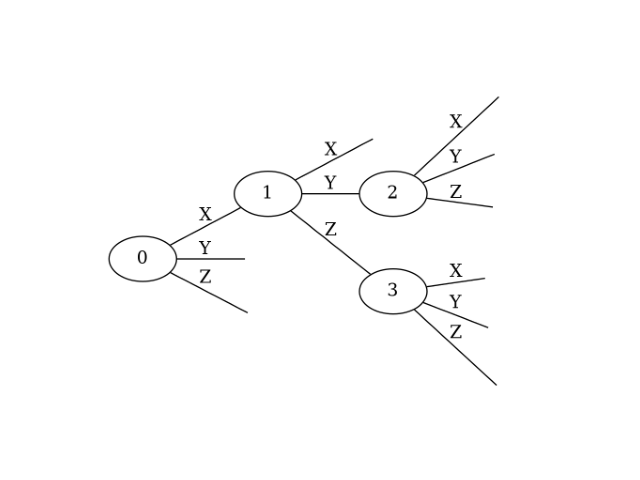
In this diagram, nodes are represented by ellipses with their numbers inside. Edges emanating from a node are labeled X, Y, or Z, corresponding to Pauli X, Y, and Z operators, respectively. Unlike general Ternary Trees, edges may not lead to a child node. For details, refer to the paper:”From fermions to Qubits: A ZX-Calculus Perspective”. The key takeaway is that any fermion-to-qubit mapping can be defined by such a Ternary Tree, and the transformation algorithm is known.

To define a Ternary Tree in yaf2q, use the TernaryTreeSpec class. Its constructor takes indices and edges arguments:

from yaf2q.ternary_tree_spec import TernaryTreeSpec

ttspec = TernaryTreeSpec(
    indices = [0, 1, 2, 3],
    edges = {1: (0, 'X'), 2: (1, 'Y'), 3: (1, 'Z')},
)

Here, indices is a list of node numbers, defining a Ternary Tree with four nodes. edges represents the set of edges. The keys are child node numbers, and the values are tuples (parent_node_number, edge_label). The root node is assumed to be 0. Child node numbers do not include 0, parent node numbers are always smaller than child node numbers, and edge tuples must be unique. This uniquely defines the Ternary Tree structure.

You can visualize the Ternary Tree using ttspec.show():

ttspec.show()

This will display the Ternary Tree diagram.

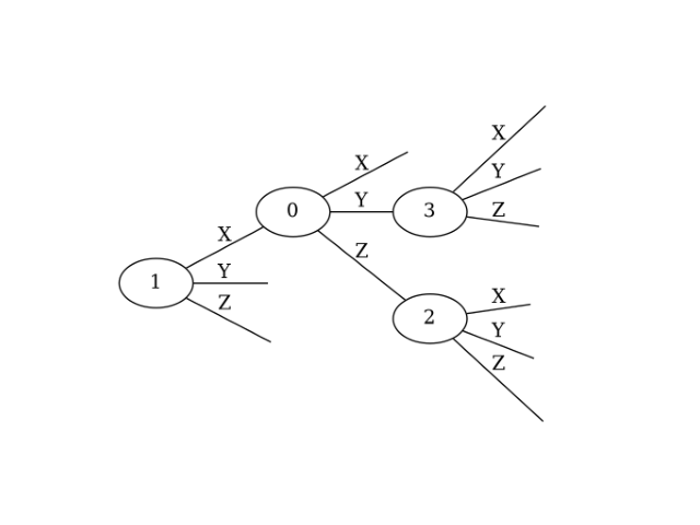
If you want to define a Ternary Tree with the same structure but different node numbering, you can reorder the indices list. Do not change edges, as this would alter the tree’s shape.

ttspec = TernaryTreeSpec(
    indices = [1, 0, 3, 2],
    edges = {1: (0, 'X'), 2: (1, 'Y'), 3: (1, 'Z')},
)
ttspec.show()

This generates a Ternary Tree with only the node numbers changed:

ternary_tree_2

You can also generate a random Ternary Tree without explicitly specifying indices and edges using the random() class method, which takes the number of nodes as an argument:

ttspec = TernaryTreeSpec.random(4)
print(ttspec)

Output:

indices:[3, 0, 2, 1], edges:{1: (0, 'Z'), 2: (0, 'Y'), 3: (2, 'Y')

Once you have a Ternary Tree, you can create an F2QMapper instance based on it:

f2q_mapper = F2QMapper(ttspec=ttspec)

From this point, you can obtain qubit states, qubit operators, and their corresponding eigenvalues, eigenvectors, and Pauli weights, just as described in the “Conventional Mapping Methods” section.

Optimizing Fermion-to-Qubit Mappings

Next, let’s discuss the optimization of fermion-to-qubit mappings.

Consider a 1D chain of four hydrogen atoms and aim to find a fermion-to-qubit mapping (i.e., a Ternary Tree) that minimizes the average Pauli weight of the resulting qubit Hamiltonian. First, create the fermion Hamiltonian using OpenFermion:

from openfermion import MolecularData
from openfermionpyscf import run_pyscf

from yaf2q.ternary_tree_spec import TernaryTreeSpec
from yaf2q.f2q_mapper import F2QMapper
from yaf2q.optimizer.sa import SAParams, SA

distance = 0.65
molecule = MolecularData(
    geometry = [('H', (0, 0, 0)), ('H', (0, 0, distance)), ('H', (0, 0, 2*distance)), ('H', (0, 0, 3*distance))],
    basis = 'sto-3g',
    multiplicity = 1,
    charge = 0,
)
molecule = run_pyscf(molecule, run_scf=1, run_fci=1)
fermion_hamiltonian = molecule.get_molecular_hamiltonian()
num_qubits = fermion_hamiltonian.one_body_tensor.shape[0]

Define an objective function that takes a TernaryTreeSpec and returns a float (e.g., the average Pauli weight). This should be defined as an inner function:

def objective_func(ttspec: TernaryTreeSpec):
    f2q_mapper = F2QMapper(ttspec=ttspec)
    qubit_hamiltonian = f2q_mapper.fermion_to_qubit_operator(fermion_hamiltonian)
    weights = qubit_hamiltonian.pauli_weights()
    weight_ave = sum(weights) / len(weights)
    return weight_ave

This function calculates the average Pauli weight. You can define any function that takes TernaryTreeSpec and returns a float. For example, you could calculate the depth of a quantum circuit for Quantum Phase Estimation and aim to minimize that.

With the objective function defined, you can use yaf2q’s SA class (Simulated Annealing) to find a solution that minimizes it. The SA constructor takes the number of qubits, the objective function, parameters (SAParams), and a verbose flag:

ttspec_opt = SA(
        num_qubits = num_qubits,
        objective_func = objective_func,
        params = SAParams(init_sampling=10, num_steps=30, cooling_factor=1.0),
        verbose = False,
).optimize()

The SAParams object controls the simulated annealing process with parameters like init_sampling (number of initial random samples), num_steps (number of annealing steps), and cooling_factor (how rapidly the temperature decreases). Default values are init_sampling=10, num_steps=10, and cooling_factor=1.0. Adjusting these parameters may be necessary for optimal convergence.

The optimize() method then executes the optimization to find an (approximately) optimal ternary tree (ttspec_opt).

Finally, use ttspec_opt to perform the fermion-to-qubit mapping and display the resulting qubit operator and Pauli weights:

print(f"* ternary tree:\n{ttspec_opt}")
f2q_mapper = F2QMapper(ttspec=ttspec_opt)
qubit_hamiltonian = f2q_mapper.fermion_to_qubit_operator(fermion_hamiltonian)
weights = qubit_hamiltonian.pauli_weights()
weight_ave = sum(weights) / len(weights)

print(f"* pauli weight (ave): {weight_ave}")

Example output:

[jordan-wigner]
* pauli wieght (ave): 4.583783783783784
[parity]
* pauli weight (ave): 4.691891891891892
[bravyi-kitaev]
* pauli weight (ave): 4.562162162162162
[ternary tree optimization]
* ternary tree:
indices:[3, 7, 2, 0, 5, 4, 1, 6], edges:{1: (0, 'Y'), 2: (1, 'Y'), 3: (2, 'Z'), 4: (3, 'Z'), 5: (4, 'Y'), 6: (3, 'X'), 7: (4, 'X')
* pauli product length (ave): 4.4324324324324325

The optimized Ternary Tree shows a smaller average Pauli weight compared to the conventional methods.

Since simulated annealing is a stochastic method, the results of the ternary tree optimization will vary. You can fix the random seed for reproducible results:

ttspec_opt = SA(
        num_qubits = num_qubits,
        objective_func = objective_func,
        params = SAParams(init_sampling=10, num_steps=30, cooling_factor=1.0, seed=123),
        verbose = False,
).optimize()